TDLAS set up and experimental results

The experimental set-up is presented in Figure 1.

Atmospheric air with water traces was flushed in the central section (8 cm long) of a heated quartz tube. A quartz tube, 30 cm long and 50 mm i.d., was located inside the electrically heated cylindrical furnace. The central section was formed between quartz wedge-shaped windows of two inserts, each 30 cm long and 40 mm i.d. A small angle between the planes of the windows minimized interference between the planes. The temperature in the central section was controlled by three commercial thermocouples PS2007 Instrument Specialists Inc., Boerne, TX, USA. The accuracy of the thermocouples was 7.5 K at 1000 K. The length of the central section was about four times less than the length of the oven providing practically uniform temperature of the gas within the section, the variation of the temperature at 1000 K was within +/− 0.3%.

Two DLs were used to probe the transitions of the H₂O molecule at 7185.6 (DL1, NEL709042) and 7466.34 cm⁻¹ (DL2, Zacher Lasertechnik 1343-05-BFY). Both DLs were stabilized and tuned by temperature (TED350) and current (LDC202) controllers (Thorlabs). A signal of a special form was additionally applied to the inputs of both controllers. This signal provided low frequency (LF) scanning of the DLs wavelengths and high frequency (HF) modulation of both DLs. The amplitudes of both LF and HF signals were optimized for both lasers independently, but LF and HF frequencies for both lasers were equal 122 Hz and 50 kHz.

The radiation of both DLs were combined in the single-mode sm splitter 1 and the mixed radiation was further split into three channels by the 3-output single-mode sm splitter 2. The first (interference) channel (3% of the radiation) was used for controlling the DLs modulation amplitude and linearization of the wavelength scale. To control the DLs scanning the radiation was delivered by the fiber s1 to the fiber Mach–Zander interferometer (etalon) with a free spectral range 0.0171 cm⁻¹. A total of 7% of the output radiation was delivered to the photodiode PDr of the second (reference) channel by fiber s2. The remaining 90% of the radiation formed the sample channel. The output of the single-mode fiber s3 was attached to the input/output of the multimode fiber m2. Then DLs radiation passed through the mm splitter, a 10 m long multimode patch cord m1 and was finally collimated by the objective on a Thorlabs F240APC-C optical collimator. The probing radiation passed through the gas cell, reflected from the micro-prism retroreflector (MPRR), focused by the same lens onto the face of fiber m1, and was delivered to the photodiode of the sample channel via the mm-splitter and fiber m3. The photodiodes Hamamatsu G8370-02 (PDi, PDr, and PDs) with a sensitive area diameter of 2 mm were used in all three channels.

The acoustic fluctuation and turbulence on the optical path of the probing DLs radiation complicated the focusing of the laser beam onto the input/output of the fiber m1. To reduce these fluctuations, the probing beam was reflected back to the detection system by micro-prism retroreflector MPRR [31]. The multimode optical fiber m1 with a 50 μm core was also used to increase the collection efficiency of the reflected probing DL beams. At the same time, its aperture was small enough to minimize the broadband thermal radiation of the hot zone of the furnace. The efficiency of the reflected radiation collection to the sample photodiode PDs was about 1%. Such low efficiency was nevertheless enough for processing the absorption signal. At the same time, the negative feedback of the reflected radiation on the performance of the DLs was negligible. The measured feedback light intensity was less than 0.1%. MPRR and focusing optics were placed in a separate box and flushed with the argon. More details on the performance of the MPRR are published elsewhere [31].

A rotating plastic disk with a specially roughened surface, which randomly modulated the laser beam transmitted intensity, was used to simulate multiplicative noise. A DC motor rotated the disk at various speeds of up to 3000 rpm.

Signals from the sample and reference channels were delivered directly to the analog logarithmic converters LC1 and LC2, based on the p-n junctions of the MAT-04 transistors (Analog Devices, subpanel in Figure 1). The amplified differential signal was demodulated by a homemade lock-in-amplifier LIA, based on an Analog Devices AD633 analog multiplier. The signal from the LIA was filtered by a low-frequency filter with a passband frequency of 3 kHz and digitized via a National Instruments NI USB-6281 data acquisition (DAQ) system.

At first, measurements were carried out in a direct absorption mode. To do this, the transistor MAT04 was replaced with a 6.2 kΩ resistor and the signal was measured at the output of the operational amplifier AD8034 (see insert in Figure 1). The modulation of the lasers was switched off. By adjusting the optical scheme, MPRR, and focusing the spherical mirror, a maximum value of the photocurrent in the measuring channel and the minimum interference effect were achieved. At a temperature of about 1000 K, the absorption signal on the 7466 cm⁻¹ line became large enough, and it could be additionally increased by introducing moist air into the central part of the cell. Then the absorption signals and the transmission spectrum of the Fabry–Perot etalon were measured simultaneously. These data were used for the linearization of the wavelength scale for both 7185 and 7466 cm⁻¹ spectral ranges.

Next, the background signal, defined by the broadband thermal radiation of the cell, backscattered radiation from the mm-fiber, and the noise in the electrical circuit, was measured with the DLs switched off. In the described system the additive signal was small enough to provide correct logarithmic processing.

At the next step, the scanning of both DLs was switched off and the signal transmitted through the cell was measured at constant DL radiation intensities. In these experiments, the output signal was measured in two modes: with the rotating disk off and on. These data were used for the evaluation of the noise spectrum in the sample channel. All further measurements were performed with the scanning and modulation of the DLs switched on. The modulation amplitude of DL2 was adjusted to maximize the signal (peak-to-peak) of the first harmonic. The amplitude of modulation of DL1 was adjusted to approximately equalize the signals of the first harmonic absorption signal registered by both DLs (7185 and 7466 cm⁻¹). This adjustment provided the correct linear performance of the LIA.

Prior to the measurements at every temperature of the cell, the optical path was flushed with argon for ~5 min. The residual water vapor in the system even after 10 minutes of argon flush, provided an absorption signal at the 7185 cm⁻¹ line above the noise level. This minimal level of 7185 signal was registered and further processed as the background signal. After registration of the background signals on both lines, ambient air was introduced into the cell and the first harmonics of the absorption signals at both lines were detected in the stationary mode. Importantly, to localize the water vapor absorption only in the cell, all parts of the flushed optical path excluding the measurement cell were maintained at the same constant level. Just after these measurements with the plastic disk off, the disk was inserted into the optical path and the measurements with the added multiplicative noise were performed.

When deriving Equation (12), we neglected the influence of the broadband illumination E(t) of the photodetector, which can be significant when working with hot objects. The presence of additional thermal radiation leads to the appearance of an additive term in the photocurrent of the sample channel:

Here, isig���� is the photocurrent of the sample channel when the broadband illumination is negligible; i_s0 = G_sτ_s(t)τ_νs(t)I₀(t); i_add is the photocurrent due to the broadband illumination; i_add = G_sE(t). In this case, the output voltage of the logarithmic converter in the sample channel is described by the equation:

As a result, an additional voltage U_add appears at the output of the differential amplifier, which for small absorptions is described by the equation:

It can be seen from Equation (17) that the illumination of the photodetector by the broadband radiation leads to a shift of the baseline at the output of the lock-in amplifier and to a decrease in the measured absorption signal by an amount proportional to i_add/i_s0. Additional illumination can also lead to errors in determining the temperature, since the values of the signal currents i_s0 in the vicinity of the two spectral lines can differ significantly. Therefore, the requirements for shielding the sample photodiode from broadband illumination become critical.

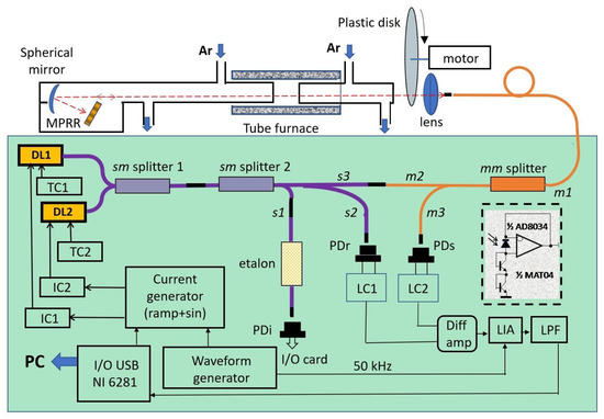
In our work, the radiation was collected in the sample channel through a multimode optical fiber with a core diameter of 50 μm. Thus, the input aperture in relation to broadband illumination was radically reduced and, accordingly, the contribution of i_add was reduced. For reliable focusing of laser radiation on the face of the fiber, the principle of autofocus using a micro-prism retroreflector was applied.

As was pointed above the errors of the logarithmic processing depend on the level of the additive component and are approximately defined by Equation (17). To check this claim, scanning (122 Hz) and modulation (50 kHz) of DL1 were switched on and the first harmonic of the absorption signal on the 7185 line was measured with logarithmic processing. At the same time, DL2 worked in a steady state mode and its radiation provided the additive input in the photocurrent of the sample photodiode PDs. The level of this additive component was maintained in the linear response mode and could be varied. The results of these measurements, presented in Table 1, confirm the validity of Equation (17). Based on the data in Table 1, one can conclude that the additive component of the current through the LC should be minimized.

In our experiments the additive contribution in the signal at 1000 K was below 3 × 10⁻³. This contribution was defined by the photocurrent from the broadband thermal radiation, the reflection of the DL radiation from the non-ideal connections in the mm-splitter, and the leakage current of the input electronic circuit cascades.

The use of LCs based on p-n junctions may introduce additional sources of uncertainties. During the modulation experiments, the errors of logarithmic processing increase with increasing modulation frequency because of leakage through the shunt capacity of the p-n junction. This capacity is defined by the eigen capacity of the junction, the input capacity of the operational amplifier, and the effective capacity of the photodiode. The capacity of a photodiode with a diameter of a sensitive area of 2 mm can be up to 1000 pF. The dynamic resistance of a p-n junction is defined by its current, and for currents less than 10 μA, this can be above several kΩ. As a result, the relation between high-frequency and low-frequency components at the output of the LC decreases compared to the input. In addition, a phase shift occurs in the high-frequency component. This effect increases with increasing modulation frequency. Significant deviations of the LC parameters from the ideal may cause additional errors in the determination of spectroscopic line parameters and, consequently, introduce errors in the determination of a gas temperature. To minimize these errors, one should use photodiodes with small eigen capacities, for example, photodiodes integrated with fibers and the radiation collection efficiency should be increased using high-quality MPRR. In our set-up, the moderate quality of all components dictated the selection of a limited modulation frequency −50 kHz. Another reason for the limitation of the modulation frequency is low efficiency of the wavelength tuning of the DLs, namely, a decrease of the modulation amplitude with increasing modulation frequency. Because of this limited efficiency, the level of RAM increases and approaches the maximum permitted level of a DL injection current.

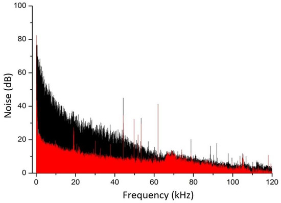
When using a rotating plastic disk (Figure 1), the mean level of photocurrent decreases by ~20% and simultaneously fluctuations sharply increase. Spectra of the photocurrent noise with (disk on, black trace) and without (disk off, red trace) the multiplicative components, measured in the direct mode are presented in Figure 2. The low frequency part of the noise spectrum with multiplicative components (black) increases by 45 dB compared to the spectrum without multiplicative components (red) and follows a 1/f dependence. Excess flicker noise exists below 60 kHz.

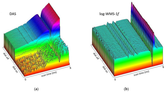
The efficiency of the new data processing algorithm is shown in Figure 3. The figure shows 3D images of raw data (signals from the photodetector PDs) registered in the DAS mode (a) and using the log-WMS-1f technique (b) for a temperature of 1050 K.

The 3D spectra registered in DAS mode exhibit well-defined absorption lines in both spectral ranges when there were no extra noises (disk off), but weak lines in the 7466 cm⁻¹ spectral range are indistinguishable in noise with the disk on. On the contrary, absorption lines in both spectral ranges are well detected even with extra noise using the log-WMS-1f technique.

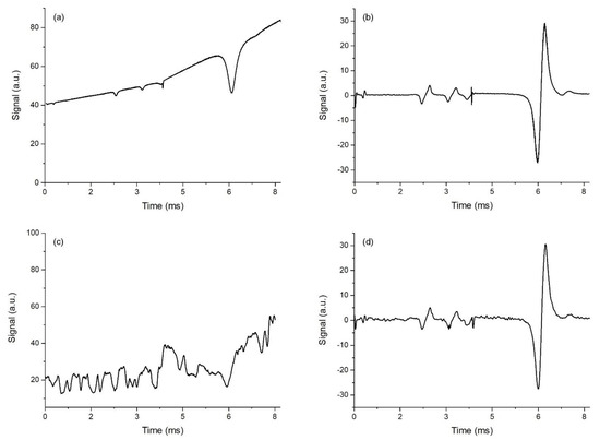
The same results were exhibited in the absorption spectra detected in a single scan. Raw data for single-scan measurements are shown in Figure 4. Signals detected in DAS mode are shown in the left panels; signals detected in the log-WMS-1f mode are shown in the right panels. The upper traces in both panels were detected without extra noise in the sample channel (disk off), while the lower traces were detected with extra noise (disk on). Large differences in the efficiency of the absorption spectra registration in the two modes were evident. The log-WMS-1f technique provided the efficient elimination of extra multiplicative noise and enables sensitive registration of weak absorption lines.

Several series of measurements were performed at temperatures ranging from 800 to 1100 K. In each series, the temperature was measured by a thermocouple and by the spectroscopic technique. The log-WMS-1f spectra were recorded without a rotating plastic disk (disk off) and with the insertion of additional multiplicative noise (disk on). At each temperature, 18 scans were recorded in one measurement. Each scan was processed separately, as well as averaged (over 18 scans) for one measurement. The amplitudes of modulation of the optical frequency of the lasers varied from series to series. Below are the results for a series in which the modulation amplitudes were set to a_m1 = 0.0057 cm⁻¹ for the 7185 cm⁻¹ laser and to a_m2 = 0.017 cm⁻¹ for the 7446 cm⁻¹ laser.

To determine the temperature, the measured spectra were fitted to a theoretical spectrum H₁(v). The absorption lines were constructed assuming a Voigt profile. Before the fitting procedure, the experimental spectra (raw data) were transformed to the frequency domain (cm⁻¹) using the measured spectrum of the Fabry–Perot etalon.

Two processing algorithms were used. The flow chart for the first algorithm is shown in Figure 5. In this algorithm, two spectral ranges (7185 and 7466 cm⁻¹) were fitted as a single spectrum. Initially, the spectrum of the first harmonic was simulated for a certain starting (guess) temperature for each section from the HITRAN database [32] according to Equation (15). The Doppler widths were fixed at a guess temperature. Fitting the simulated spectrum to the experimental one was carried out using the nonlinear least squares method. Least squares (model fitting) algorithms [33] were employed. In each range, the fitting parameters were the positions of the centers of the absorption lines ν₀₁, ν₀₂, and their Lorentzian widths Δν_L1 and Δν_L2. The common fitting parameters in the two ranges were temperature T and coefficient K. As suggested in [34], the contribution of the first three orthogonal polynomials was additionally subtracted from the experimental and simulated spectra. From a mathematical point of view, this was equivalent to fitting the baseline of the experimental spectra using a parabola [35].

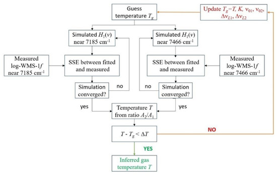
The flow chart for the second fitting algorithm is shown in Figure 6. In this algorithm, the simulated spectrum H₁(v) was fitted separately for each spectral range. At the initial (guess) temperature T_g, the line absorbance A₁ and A₂ were determined independently for the position of the line centers ν₀₁ и ν₀₂, the Lorentzian widths of the lines Δν_L1, Δν_L2, and the coefficient K. Temperature T was inferred using Equation (4). If T was noticeably different from T_g, then an iterative procedure was started. Iterations were stopped when the difference in temperature evaluation between two successive steps was less than 10 K. This temperature was assumed as the measured gas temperature in the cell.

As an example, Figure 7 shows the spectra measured in one scan for T = 1050 K (thermocouple) and the residuals from processing using the first algorithm. The developed log-WMS-1f technique provides a very reasonable estimation of the gas temperature, even in one scan. Note that the laser was scanned with a frequency of 122 Hz, which gives an estimation of the temporal resolution of about 8 ms. The temperature obtained as a result of fitting was T = 1022 K for the disk off. For the experiments with additional noise (disk on) the temperature inferred from the “noisy” spectra was T = 1040 K. Fitting using the second algorithm gave 1043 and 1057 K, respectively.

The results of fitting of all scans from this series of experiments for temperature T = 1050 K (thermocouple) are shown in Figure 8. Each point in Figure 8 is the T value obtained in a particular scan when processed by two algorithms and with the disk off/on (see the legend to the figure). In some scans, the deviations from the temperature of the thermocouple were larger with noise, and in some without noise. The values for three temperatures averaged over 18 scans and according to statistical errors for different modes (disk off/on) and different processing algorithms are presented in Table 2. These results show that statistical errors in the case of noise were greater than those without noise. Nevertheless, due to the good noise suppression by our proposed method, the temperature estimate was quite good even in the presence of excessive noise.

Experiments were performed with the plastic disk off (without extra noise) and on (with extra noise). The temperature was evaluated using two algorithms of data processing. For all series of experiments conducted the difference between the temperature measured by a standard thermocouple and the average value determined by the developed methods was, with the disk turned on, ΔT ≤ 40 K for temperature ~1000 and ΔT ≤ 30 K for temperature ~800 K.

The results presented in Table 2 show that both algorithms of data processing provided quite close temperature estimates. Generally, the second one was better for the case of the large difference in the intensities of absorption lines, while in the process of separate fitting the strong line did not “impose” its line shape on the weak one. In our review [35], we discussed the situation with lines of comparable intensity when both algorithms were equivalent. In the current paper, the lines were very different, and it was better to use the second algorithm. The first algorithm can be used in the case of registration of both lines within the tuning range of one DL [9,13]. In this situation, the simultaneous fitting of lines of comparable intensity will allow a better approximation of the baseline.