

https://doi.org/10.1038/s41598-022-27057-2
”
Atomic force microscopy (AFM) is a unique technique for imaging structures of sample molecules bound to a surface at ambient conditions1. Recently, high-speed AFM (HS-AFM) with dramatically faster imaging rates (up to tens of frames per second) has been developed, enabling us to directly observe biomolecules in action2,3. HS-AFM can investigate detailed structure–function relationships in biomolecules that cannot be observed with other methods, and it has been established as one of indispensable techniques in modern biophysics. Example applications of HS-AFM include myosin V walking along an actin filament4, rotary catalysis of F1-ATPase5, structural dynamics of intrinsically disordered protein6, and the functional dynamics of CRISPR-Cas9 in action7. Currently, the spatial resolutions of HS-AFM instruments are ~ 2 nm in the lateral direction and ~ 0.15 nm in the vertical direction to the AFM stage8.
Importantly, separately from the resolution of the image profile, the resolutions of the obtained sample surface information are further limited by the tip geometry and the tip-sample interactions. The relationship among the tip geometry, the image profile, and the sample surface is shown in Fig. 1a and b. When the tip is sufficiently thin, the obtained image profile is nearly the same as the sample surface (Fig. 1a). On the other hand, when the tip is blunt compared to the scale of samples, the image profile is blurred from the sample surface (Fig. 1b). Once the tip shape is known, algorithms, called erosion, have been proposed to “deconvolve” the image profile for reconstructing approximate sample surface geometry9,10,11. Thus, to reconstruct the surface geometry of the sample molecule, it is crucial to know the tip shape accurately. Tip shape estimation is also important for inferring 3D molecular structures from AFM images. In the recent analysis of AFM images, pseudo-AFM images are emulated from 3D molecular structures (obtained with different experimental or computational techniques, e.g., X-ray crystallography or molecular dynamics simulations) and an assumed tip shape and then compared with the experimental AFM image12,13,14,15,16,17,18,19,20,21. In the analysis, the 3D structure which generates the pseudo-AFM images most similar to the experimental AFM image is selected as the best estimate for 3D molecular structure. In this kind of analysis, the accuracy of pseudo-AFM images crucially depends on the tip shape. Thus, the tip shape should be determined as accurately as possible.
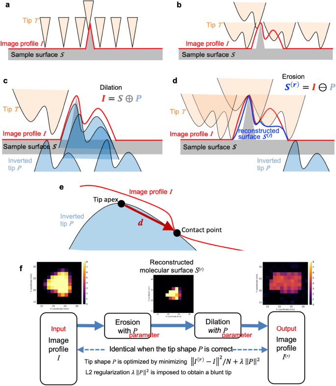
Morphology operators and schematic of end-to-end differentiable blind tip reconstruction (BTR). (a) Image profile obtained by scanning a surface with a thin tip. (b) Image profile obtained by scanning the same surface as (a) with a blunt tip. (c) Schematic picture illustrating a morphology operator, dilation. (d) Schematic picture illustrating a morphology operator, erosion. Here, for the sake of intuitive explanation, erosion is represented with a non-inverted tip instead of its inversion. (e) Relation of a contact point and tip apex position, explaining the idea behind the original BTR. (f) Schematic of end-to-end differentiable BTR.
Currently, there are three possible approaches to obtain a tip shape22,23. The first approach is the direct imaging of a tip using either a scanning or transmission electron microscope (SEM or TEM). However, both SEM and TEM provide only a two-dimensional projection of the sample. It is unrealistic to install special equipment for imaging the tip from various angles as a routine for determining the tip shape. Moreover, as the tip can be damaged over time during AFM measurement, determining tip shape before or after the AFM measurement is not necessarily appropriate. The second approach is to estimate the tip shape during the AFM measurement. This approach determines the tip shape from samples whose geometry is a priori known24,25,26. With the combination of mathematical modeling, an approximate tip shape can be reconstructed. For example, Niina et al. recently proposed a method to estimate a tip shape by comparing the pseudo-AFM images generated from 3D molecular structures with AFM images20. By assuming that the tip shape is a hemisphere (radius r) combined with a circular frustum of a cone (half angle θ), they proposed to estimate these two geometric parameters. However, since real tips can be of any shape, e.g., double-tip shape with two separate acutes, the assumption of a shape limits the application of the method.
The third approach estimates the tip shape through the image analysis of AFM data without any prior knowledge of sample molecule and tip shape. The blind tip reconstruction9 developed by Villarrubia is a classical method to estimate arbitrary tip shapes from AFM images. The idea behind the algorithm is to recognize that sizes and depths of dents in the image profile must be smoother than the sharpness of the tip. Then, the algorithm “carves” an initially blunt tip according to the sizes and depths of dents (details will be described below). While the BTR works perfectly for noise-free AFM images, its algorithm is susceptible to noise, or it is difficult to determine a threshold parameter against noise. This is a crucial issue for the analysis of HS-AFM images because HS-AFM is generally more prone to noise than conventional AFM. Over these two decades, several improvements or new methods have been proposed for better estimation of tip shape; Dongmo et al. proposed monitoring tip volume for tuning thresh parameter for noisy AFM images. Tian et al. extended Villarrubia’s original BTR with the dexel representation for reconstructing general 3D tip shapes and proposed an improved regularization scheme against noise27. Jóźwiak et al. simplified Tian’s idea to the case of standard AFM tips28. Flater et al. proposed a systematic way to determine the threshold parameter against noisy AFM images22. By approximating mathematical morphology operators by linear operators, Bakucz et al. proposed a reconstruction method based on the Expectation–Maximization (EM) algorithm with the tip shape represented as a hidden variable29. Despite these studies, the original BTR is not routinely utilized in the analysis of noisy AFM data, especially for the analysis of HS-AFM data, due to its susceptibility to noise and difficulty in tuning the parameter.
The reason why Villarrubia’s BTR is susceptible to noise is that it is difficult to correctly determine whether the tip shape geometry or noise causes an individual dent in the image profile. In the algorithm of the BTR, once a dent caused by noise is misinterpreted as the cause of the geometry of the tip, the tip is “carved” to be fitted to the noise. This leads to a reconstruction of very thin tip shape. In terms of machine learning theory, this can be regarded as overfitting the tip shape to noise.
To prevent such overfitting, we here introduce an appropriate loss function including a regularization term considering noise statistics, which are absent in the original BTR. As the morphology operators (Fig. 1c,d) used in the loss function are complicated nonlinear functions, minimizing such a complicated loss function over tip shape is challenging. The technologies developed by recent advances in deep learning studies30 can potentially overcome this problem. Automatic differentiation and smart optimizers are recently being applied to optimize not only the parameters of neural networks but also the parameters of physical models, by implementing physical functions as differentiable functions31,32. For example, Zhou et al. recently modeled the Lorentz TEM observation process as a differentiable neural network layer and successfully solved the inverse problem of phase retrieval stably by backpropagation33. In the current study, we propose to use these technologies to optimize the loss function over the tip shape. Our method (called the end-to-end differentiable BTR) implements morphology operators as differentiable functions and optimizes the loss function in the same way as neural networks under a deep learning framework. Using pseudo-AFM images generated from a known molecular structure (myosin V motor domain) as a test case, we show that the differentiable BTR is robust against noise in AFM images, as well as lower parameter dependence compared to the original BTR. Furthermore, the differentiable BTR can correctly detect double tips, one of the artifacts that frequently occur in AFM measurements. Finally, we applied the method to real noisy HS-AFM images, myosin V walking along an actin filament.
“