A Quantitative Method for the Composition of 7B05 Cast-Rolled Aluminum Alloys Based on Micro-Beam X-ray Fluorescence Spectroscopy and Its Application in Element Segregation of Recrystallization

https://doi.org/10.3390/ma16041605

“Microscopic content segregation is among the important reasons for the anisotropy of mechanical properties in the cast-rolled sheets of the 7B05 aluminum alloy. It is of great significance to study the uniformity of aluminum alloys in terms of the microscopic composition and structure. In this study, a precise method for composition quantification based on micro-beam X-ray fluorescence spectroscopy is established by parameter optimization and a calibration coefficient. Furthermore, this method was applied for exploring and quantifying the relationship between recrystallization and deformation microstructures. The results show that the comprehensive measurement effects of all elements are the best when the X-ray tube voltage is 50 kV, the current is 150 μA, and the single-pixel scanning time is 100 ms. After verification, the sum of differences between the measured values and the standard values for all elements using the calibration coefficient is only 0.107%, which confirms the accuracy of the optimized quantitative method. Three types of segregation indexes in national standards were used to capture small differences, and finally ensure that the segregation degrees of elements are Ti > Fe > Cr > Cu > Mn > Zr > Zn > Al. The quantitative segregation results obtained by the spatial-mapping method show that the difference in the content of Al and Zn is approximately 0.2% between the recrystallization region and the deformation region, the difference in the content of Fe and Ti is 0.018% and 0.013%, the difference in the content of Cr, Cu and Zr is approximately 0.01%, and the difference in the content of Mn is not obvious, only 0.004%.”

2.2. Instruments and Conditions of Composition Test

Figure 2. Schematic diagram of the structure of the micro-beam X-ray fluorescence spectrometer.

3.3. Application of Composition Analysis Method in the Aluminum Alloy

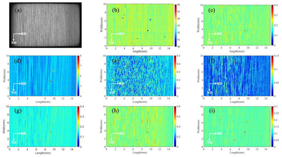
The quantitative analysis of each element in the range of 15 mm × 10 mm is carried out using the optimized quantitative method. In this method, the X direction is the thickness direction, and the number of component arrays is 1440 rows; the Y direction is the length direction, and the number of component arrays is 840 columns. The two-dimensional component distribution is shown in Figure 7. The results show that there are differences in the distribution of elements along the thickness direction of the rolled aluminum alloy plate—the distribution of elements in the surface layer is relatively uniform, and the distribution in the central layer presents a band-like segregation with a similar shape to that of the corroded structure.

Figure 7. Two-dimensional distribution map of element content in 7B05 aluminum alloy; (a) metallographic structure after corrosion, (b) Al, (c) Cr, (d) Zn, (e) Fe, (f) Ti, (g) Cu, (h) Mn, and (i) Zr.

In accordance with the GB/T24213-2009 on general rules of original position statistics, the content distribution analysis of each element at different positions obtained from the surface distribution was carried out. Statistical parameters such as the degree of segregation degree, statistical segregation degree, and segregation ratio of each element in the entire scanning area are obtained. For values of S and SRx, refer to Equations (1) and (3). Values of DS Positive and DS Negative correspond to confidence intervals of 97.5% and 2.5%, respectively, referring to Equation (2). The results are shown in Table 5.

Table 5. Results of statistical distribution analysis of element content.

Index/Element	Al	Cr	Cu	Fe	Mn	Ti	Zn	Zr
Average	93.12 ± 0.188	0.21 ± 0.003	0.15 ± 0.004	0.19 ± 0.014	0.39 ± 0.013	0.04 ± 0.004	4.31 ± 0.146	0.14 ± 0.005
Maximum (97.5%)	93.77	0.25	0.18	0.34	0.48	0.08	4.59	0.17
Minimum (2.5%)	92.24	0.17	0.12	0.09	0.33	0.01	4.03	0.12
S	0.008	0.204	0.201	0.692	0.203	0.946	0.0653	0.175
DS Positive	0.007	0.200	0.188	0.765	0.244	1.000	0.065	0.214
DS Negative	−0.009	−0.200	−0.188	−0.529	−0.146	−0.750	−0.065	−0.143
SRx	1.014	1.38	1.374	2.841	1.344	5.182	1.116	1.317

Three different statistical methods are chosen to quantitatively compare the segregation degree of elements: S, SR_x, DS Positive and DS Negative, as shown in Table 5. This table indicates S: Ti > Fe > Cr > Mn > Cu > Zr > Zn > Al; SR_x: Ti > Fe > Cr > Cu > Mn > Zr > Zn > Al; DS Positive: Ti > Fe > Mn > Zr > Cr > Cu > Zn > Al; DS Negative: Ti > Fe > Cr > Cu > Mn > Zr > Zn > Al. The above four segregation indicators show that the segregation of Ti is the most serious, followed by Fe, and the distributions of Al, Zn, and Zr are the most uniform. The segregation degrees of Cr, Cu and Mn are similar, the S indicates that three elements are difficult to separate (0.204, 0.201, 0.203), and the SR_x and DS Negative indicates that three elements are relatively different. In summary, the results of four segregation evaluation indexes are basically consistent, which can be used to characterize small segregation difference in a complementary manner; the segregation degree of element in 7B05 is Ti > Fe > Cr > Cu > Mn > Zr > Zn > Al.

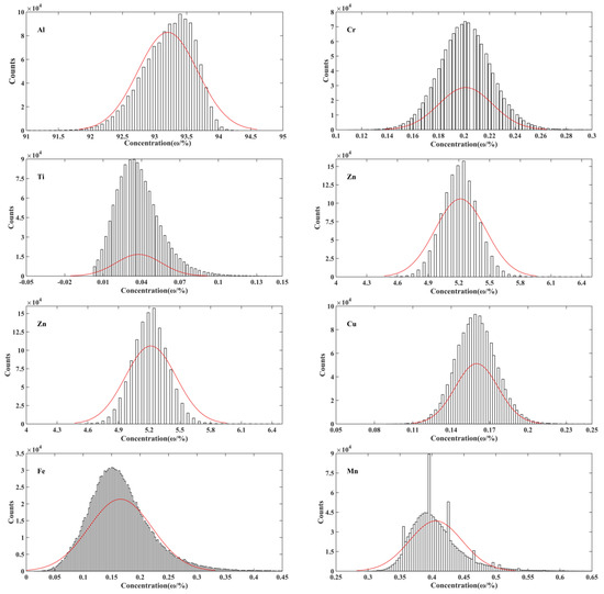
The frequency distribution diagram of element content is shown in Figure 8. The red curve is the normal distribution fitted by the frequency distribution map of each element, and the sparseness of the map is related to the total categories of content values. It can be seen from the figure that the frequency distribution basically conforms to the normal distribution, and the distribution of Al, Fe and Mn has a larger deviation from the normal distribution curve. Al has a tailing effect at low content, the total number of low content points higher than that of high content points. The number of Fe and Mn with high content points is more than that of lower content points, which may be related to the point-like segregation generated by the second phase in the cross section. The normal distribution curve of Ti has the flattest amplitude, indicating that the data distribution of Ti is more discrete from the average, and the data fluctuation is the largest. It is consistent with the calculated results of statistical segregation degree.

Figure 8. The frequency distribution histogram of element content in the 7B05 aluminum alloy.

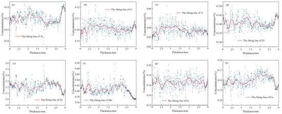
Furthermore, to explore the variation law of the content along the thickness direction in the aluminum alloy rolled sheet, the scatter diagram and fitting diagram of the average content are shown in Figure 9. As can be seen from Section 3.3, the mapping data in the section consist of 1440 columns and 840 rows. The average data of 840 rows corresponding to each column were extracted, and a total of 1440 data points were obtained along the thickness direction. Each point represents the average value of 840 rows and 1 column, which means each point represents the average content of 840 μm × 10 μm microdomains. The figure reveals that from the center of the rolled sheet to the left and right surfaces, the distribution of elements is asymmetric, and the overall content fluctuates greatly, but the element fluctuation is relatively small in the range of 5–1 mm. There is some connection in the distribution of elements. The regularities of Al and Zn elements show opposite trends, and the changing trends of Al and Cr, Zn and Fe, Cu and Ti are similar.

Figure 9. The average content line distribution along the thickness in the 7B05 aluminum alloy rolling plate; (a) Al, (b) Cr, (c) Ti, (d) Zr, (e) Zn, (f) Mn, (g) Fe, (h) Cu.